2. SINGLE POLE

About This System

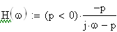
This system is about as simple as they come (other than a constant gain). It's not exciting, but you have to walk before you can run. The transfer function below is set up to give unit gain at DC:

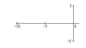
where p is the pole location (normally left half plane, so stable)

A few systems that have transfer functions of this type (i.e., single time constant) are shown below:

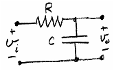
RC lowpass: input v_i, output v_o

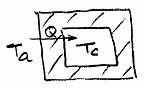
thermally insulated chamber: input T_a (ambient temperature), output T_c (chamber temperature)

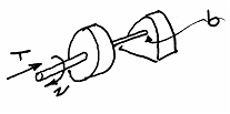
flywheel with viscous friction coefficient b: input T (torque), output n (rotational speed of the shaft)

Animated Responses

For the animation, we'll start with a large negative value of the pole location p and sweep it to the origin and just into the right half plane. In the right half plane, the impulse and step responses show the system to be unstable, so there is no defined frequency response. Click here to see the animation, and leave the animation window open as you read this section. Drag the animation slider back and forth with your mouse to get different parameter values and change all the graphs together.

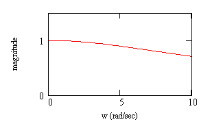
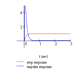
This system has a lowpass characteristic. Note that the time constant is the reciprocal of the bandwidth and the negative reciprocal of the pole location t = -1/p. As the pole becomes closer to the origin, the bandwidth of the system decreases and the time constant increases; that is, it responds more slowly to the input and starts its attenuation at lower frequencies. A pole well out from the origin produces a wider bandwidth and faster response (shorter time constant) - the step response looks more like a step itself and the impulse response begins to look like an impulse itself.

Uses

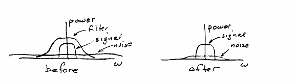
In electronics, this type of filter is frequently used to smooth signals by suppressing rapidly-varying noise or to extract a low frequency signal from high-frequency interference.

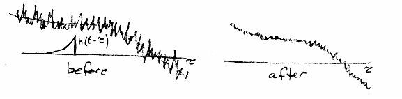
• Time-domain explanation: rapidly varying noise averages out to almost zero in the convolution integration, since h(t) is fairly smooth and slowly varying, whereas the even more slowly varying desired signal is relatively unaffected.

• Frequency-domain explanation: rapid variation in the noise implies that a significant portion of its power is at higher frequencies, which are attenuated by the filter. The desired signal varies slowly, so its frequencies are within the bandwidth of the filter. Of course, this is a pretty crude lowpass, so selection of the pole location requires a tradeoff between distortion of the signal and suppression of the noise.

=========================================================

Work Area

Here you can make your own animation, with your own parameter choices.

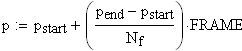
(number of frames in animation)

FRAME is the frame counter variable, an integer that will run from 0 to N_f.

the time constant in seconds

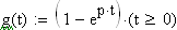
step response, also written as 1 - e^-t/t , forced to be causal

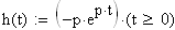
impulse response, also written as (1/t) e^-t/t, forced to be causal

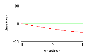
frequency response (set to zero if pole not in LHP)

Here's how to animate the plots below. From the menu, View Animate. In the resulting dialog box, select the FRAME range from 0 to 40 at 10 frames/sec. Next use your mouse to enclose all the graphs and the values of p and t in a dotted selection box, then click the Animate button in the dialog box. After an interval of computation, during which you see a thumbnail of the animation, Mathcad pops up a window with your animation. You can resize the window if you like, then play it. It's even more informative to pull the slider back and forth with the mouse, so you can change all the graphs together at your leisure.

single time constant (1 real pole)

.

.