5. TWO REAL POLES AND A ZERO
About This System
What do you get if you cascade the unit gain
lowpass circuit
of Section 1 and the unit gain
highpass circuit
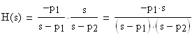
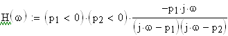
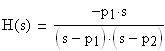
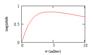
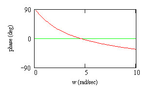
of Section 2? What's left if you cut out the low frequencies and the high frequencies? Answer: you're left with the midrange, and the composite circuit is a bandpass filter. Here's the transfer function, with p1 as the lowpass pole and p2 as the highpass pole.
H(s) is not normalized to unit gain in this formulation; in fact, the gain varies with pole location up to a mazimum of unity in the midrange if the poles are far apart.
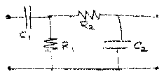
Here are a couple of circuits that are described by a transfer function of this form. Note that the poles of the left hand circuit are not -1/R1C1 and -1/R2C2, the poles of the two sections individually, because the second section loads the first (i.e., drains current from it), thereby shifting the pole location. As in the
two real pole circuit
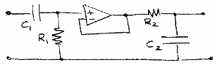
of Section 4, you can use an op amp to make the transfer function equal to the product of the section transfer functions, if this is important to you.
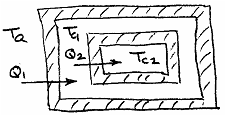
The third example is a thermal system in which the output is the temperature Tc1 in the outer chamber in response to changes in the ambient temperature Ta.
Animated Responses
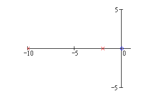
For the animation, we'll start with a large negative value of one of the poles and sweep it in to the origin, while the zero and the other pole remain fixed. The moving pole doesn't go into the right half plane, even though unstable systems still have step and impulse responses. Click
here
to see the animation and leave the animation window open as you read this section. Drag the slider back and forth with your mouse to get different parameter values and change all the graphs together.
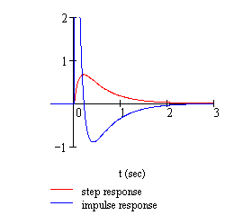
Remember that time constants are negative reciprocals of the pole locations (e.g., t1 = -1/p1). You can see two different time constants when the poles are widely separated.
Uses
This is the simplest and cheapest form of bandpass filter. Clearly, it cuts out DC and very high frequencies, but the variation in H(w) means that only signals occupying a restricted range of frequencies will get through without appreciable distortion. The pole location must be chosen intelligently, since lowpassing a highpassed signal could result in a "no pass" filter - for example, when the lowpass pole p1 is closer to the origin than the highpass pole p2, as you saw at the end of the animation
The circuit is commonly used in demodulation of a bandpass signal: multiplication of the signal by a sine wave at the carrier frequency results in a component at or near 0 Hz and a component at twice the carrier frequency. Applying this circuit to the product eliminates the double frequency term and cuts out any DC bias.
============================================================
Work Area
Make your own animation below.
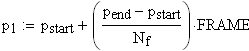
Set the pole and zero locations:
sweep the lowpass bandwidth down from high frequencies to low:
(number of frames in animation)
FRAME is the frame counter variable
fixed position of the other pole (change it, if you like)
postion of the zero (at the origin)
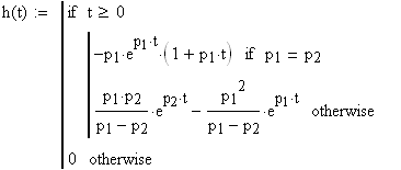
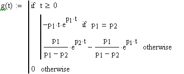
In defining the impulse and step responses, we have to allow for the possibility that p1=p2, since a double pole produces a different functional form of the solution, one that sidesteps the division by zero that would result from use of the standard form. Both of these expressions were obtained by performing an inverse Laplace transform.
set to zero if unstable
Now animate the plots and text below (use FRAME from 0 to 40):
two real poles and a zero
.