State Space Equation:

The state-space representation of a system is usually much easier to derive from the differential equations than Laplace transform method. Difficulties arise when the derivatives of the inputs appear in the differential equations, and this situation occurs here, which leads to a lot of algebra. The dynamic equations of the bus and suspension mass are:

To be a valid state-space representation, the derivative of all states must be in term of inputs and the states themselves. At the moment we have not even determined what are good states to use. To begin, divide the first and second equations by M1 and M2 respectively. Note appears in the equation for .

The first state will be X1. Since the derivative of the inputs does not appear in the equation for , choose the second state to be . We then choose the third state to be the difference between X1 and X2. After doing some algebra, we will determine what the fourth state should be. So we substitute the third state, Y1 = X1-X2, in the above equations:

Subtract the second equation from the first equation to get an expression for :

Since we cannot use second derivatives in the state-space representation, so we integrate this equation to get :

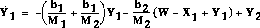
No derivatives of the input appear in this equation, and is expressed in terms of states and inputs only (since X2 = X1-Y1), except for the integral. Call the integral Y2. The state equation for Y2 is:

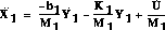
Substitute X2 = X1-Y1 in to get the state equation for Y1:

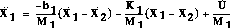
Then substitute the derivative of Y1 into the equation of the derivative of X1 :

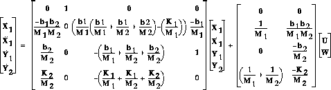
The state variables are X1,,Y1, and Y2. The matrix form of the above equations is.

The method use to find the state-space for this problem is an integral method, which was trick. For most problems, however the state-space method is much easier than the Laplace transform method.

Entering equations into Matlab

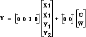
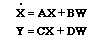
We can put the above space-form equations into Matlab by defining the four matrices, A, B, C, and D, of the standard state-space equation

 
m1=2500;
m2=320;
k1 = 80000;
k2 = 500000;
b1 = 350;
b2 = 15020;

A=[0                 1   0                                              0
  -(b1*b2)/(m1*m2)   0   ((b1/m1)*((b1/m1)+(b1/m2)+(b2/m2)))-(k1/m1)   
-(b1/m1)   
   b2/m2             0  -((b1/m1)+(b1/m2)+(b2/m2))                      1
   k2/m2             0  -((k1/m1)+(k1/m2)+(k2/m2))                      
0]; 
B=[0                 0
   1/m1              (b1*b2)/(m1*m2)
   0                -(b2/m2)
   (1/m1)+(1/m2)    -(k2/m2)];
C=[0   0   1   0];
D=[0    0];

Open-loop response

We can use Matlab to display how the original open-loop system performs(without any feedback control). Add the following command into the m-file and run it in the Matlab command window to see the response for unit step actuated force input and the response to a 0.1 m high step disturbance input.

step(A, B, C, D, 1) 

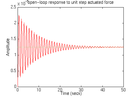
From this graph of open-loop response for unit step actuated force, we can see that the system is under-damped, when the unit step actuated force is applied. People sitting in the bus will feel a very small amount of oscillation and the steady-state error is about 0.013 mm. Moreover, the bus takes an unacceptably long time to reach the steady state. The solution to this problem is to add a feedback controller into the system's block diagram.

Note that the B matrix has been multiplied by 0.1 to simulate a 10 cm high step.

step(A, 0.1*B, C, D,  2) 

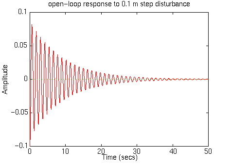
To see some details, you can change the axis:

axis([0 10 -.1 .1])

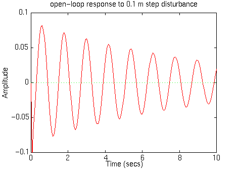
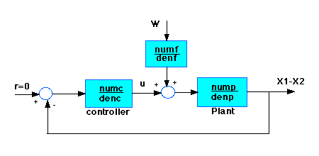
From the transfer function in Matlab command, we also can add the following commands into the m-file and run in Matlab to see the response of the unit step From this figure we see that when the bus passes a 10 cm bump on the road, the bus body will oscillate for an unacceptably long time. People sitting in the bus will not be comfortable with such an oscillation. The big overshoot (from the impact itself) and the slow settling time will cause damage to the suspension system. The solution to this problem is to add a feedback controller into the system to improve the performance. The schematic of the closed-loop system is the following:

Converting State Space to Transfer Function

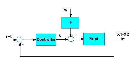
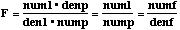
Before we start designing the controller, let's first find the transfer functions for the Plant and the disturbance transfer function, F respectively. We can find the transfer function of the plant (from the input u to the output X1-X2) by Matlab using the ss2tf command. Add the following code into your m-file:

[nump,denp]=ss2tf(A,0.1*B, C, D, 1)

The 1 indicates which input should be used to compute the transfer function. Rerun the m-file and you should get the results from your Matlab command window as the following:

nump =

      0    0.0000    0.0035    0.0188    0.6250
denp =

    1.0e+04 *

      0.0001    0.0048    0.1851    0.1721    5.0000

Note that the numerator polynomial of 5th order with two leading zeros. This may get us some trouble in the future when we add a controller to the system. When the numerator is combined with the controller numerator, the two leading zeros may increase the order of magnitude of the closed-loop numerator polynomial so that it is of higher order than the denominator polynomial. This situation is not allowed by Matlab and will result in an error. Click here and read about transforming state-space equations to transfer functions to learn more about this problem. To eliminate these two digits, redefine the num to be only the last three digits by adding the following text into the m-file:

nump=[nump(3) nump(4) nump(5)]

Therefore the transfer function of Plant become:

Plant = nump/denp

Now we know the transfer function of the plant is nump/denp, but what is the transfer function of F? First we need to find out the transfer function from the input W to the output X1-X2 by using the ss2tf command:

[num1,den1]=ss2tf(A,0.1*B,C,D,2)

Note that 2 is used to find the transfer function from the second (disturbance) input and 0.1 corresponds to 10 cm step input. Matlab should return:

num1 =

   1.0e+03 *

          0   -0.0469   -1.5625    0.0000    0.0000     

den1 =

   1.0e+04 *

     0.0001    0.0048    0.1851    0.1721    5.0000

Add the following lines into your m-file:

num1=[num1(2) num1(3) num1(4) num1(5)];

From the schematic above we see that F * Plant=num1/den1, so that F=num1/(den1*Plant), or:

The transfer function for the feedback loop,numc/denc, is the only thing left that we have to find to satisfy the specification of the bus system.

Therefore the bus-system block diagram becomes:

---

Use your browser's "Back" button to return to the previous page.

6/25/97 PP