Type 1 Systems Examples
Let's say that we have a system that looks like this:

where G(s) is:
1
-----------------
s (s + 2)(s + 3)
Let's look at the closed-loop response for this system when we use different inputs:
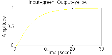
Step Input
num = 1;
den = conv([1 2],[1 3]);
den = conv(den,[1 0]);
[clnum,clden] = cloop(num,den);
step(clnum,clden)

Our steady-state error is zero.
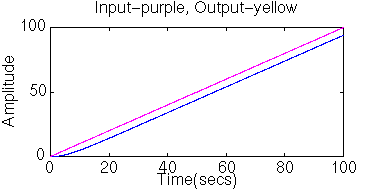
Ramp Input
num = 1;
den = conv([1 2],[1 3]);
den = conv(den,[1 0]);
[clnum,clden] = cloop(num,den);
t = 0:0.1:100;
u = t;
[y,x] = lsim(clnum,clden,u,t);
plot(t,y,t,u)
xlabel('Time(secs)')
ylabel('Amplitude')
title('Input-purple, Output-yellow')

Our steady-state error is a constant.
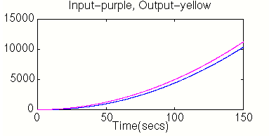
Parabolic Input
num = 1;
den = conv([1 2],[1 3]);
den = conv(den,[1 0]);
[clnum,clden] = cloop(num,den);
t = 0:0.1:150;
u = 0.5*t.*t;
[y,x] = lsim(clnum,clden,u,t);
plot(t,y,t,u)
xlabel('Time(secs)')
ylabel('Amplitude')
title('Input-purple, Output-yellow')

Our steady-state error is infinity (the error continually increases as time goes to infinity).
Use your browser "Back" button to return to the previous page
8/28/96 LJO


