Type 2 Systems Examples
Let's say that we have a system that looks like this:

where G(s) is:
(s + 1) (s + 3)
-------------------
s^2 (s + 2)(s + 3)
Note that we are using a different numerator in our transfer function in order to make sure we have a stable closed-loop system
Let's look at the closed-loop response for this system when we use different inputs:
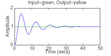
Step Input
num = conv([1 1],[1 3]);
den = conv([1 2],[1 3]);
den = conv(den,[1 0]);
den = conv(den,[1 0]);
[clnum,clden] = cloop(num,den);
step(clnum,clden)

Our steady-state error is zero.
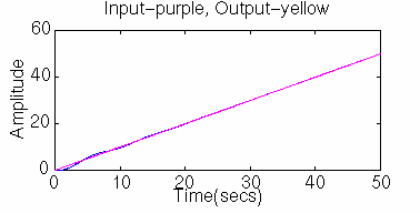
Ramp Input
num = conv([1 1],[1 3]);
den = conv([1 2],[1 3]);
den = conv(den,[1 0]);
den = conv(den,[1 0]);
[clnum,clden] = cloop(num,den);
t = 0:0.1:50;
u = t;
[y,x] = lsim(clnum,clden,u,t);
plot(t,y,t,u)
xlabel('Time(secs)')
ylabel('Amplitude')
title('Input-purple, Output-yellow')

Our steady-state error is zero.
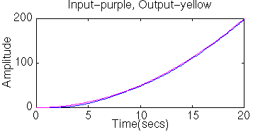
Parabolic Input
num = conv([1 1],[1 3]);
den = conv([1 2],[1 3]);
den = conv(den,[1 0]);
den = conv(den,[1 0]);
[clnum,clden] = cloop(num,den);
t = 0:0.1:20;
u = 0.5*t.*t;
[y,x] = lsim(clnum,clden,u,t);
plot(t,y,t,u)
xlabel('Time(secs)')
ylabel('Amplitude')
title('Input-purple, Output-yellow')

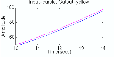
Our steady-state error is constant, but it's kind of hard to see. Therefore, we will zoom in to show this steady-state error:

Use your browser "Back" button to return to the previous page
8/28/96 LJO


