

|
|
Let's zoom in on the Nyquist diagrams corresponding to different gains using the zoom command.
nyquist(4.5*50, [1 9 30 40])
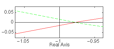
Note that the Nyquist diagram does not encircle the -1 point.
We will now look at our step response. Remember that we must look at the closed-loop step response.
k =4.5;
num = 50;
den = [1 9 30 40];
[num1, den1] = cloop (k*num,den);
step(num1,den1)
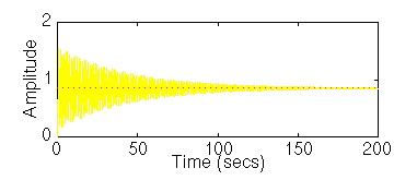
The system is stable.
nyquist(4.6*50, [1 9 30 40])
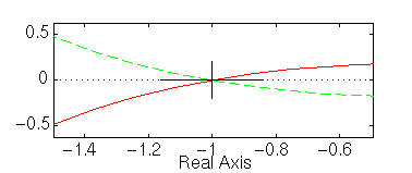
Note that the Nyquist diagram goes right through the -1 point.
We will now look at our step response. Remember that we must look at the closed-loop step response.
k =4.5;
num = 50;
den = [1 9 30 40];
[num1, den1] = cloop (k*num,den);
step(num1,den1)
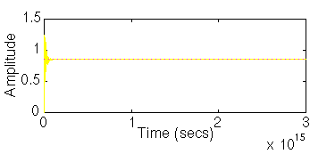
The system is marginally stable (Note the time axis).
nyquist(4.7*50, [1 9 30 40])
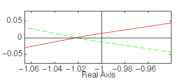
Note that the Nyquist diagram encircles the -1 point.
We will now look at our step response. Remember that we must look at the closed-loop step response.
k =4.7;
num = 50;
den = [1 9 30 40];
[num1, den1] = cloop (k*num,den);
step(num1,den1)
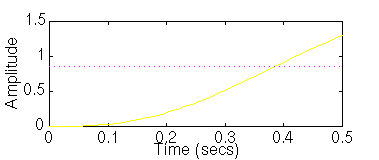
The system is unstable.
Use your browser "Back" button to return to the previous page
8/27/96 LJO