Introduction
DC behaviour of electronic circuits is described by systems of non-linear algebraic equations whose solutions are known as circuit’s DC operating points. DC operating points are usually calculated by using the Newton-Raphson method or its variants such as damped Newton methods. These methods are robust and have quadratic convergence when a starting point sufficiently close to a solution is supplied. The Newton-Raphson algorithms sometimes fail because it is difficult to provide a starting point sufficiently close to an often unknown solution. Computational difficulties in computing the DC operating points of transistor circuits are exacerbated by the exponential nature of the diode-type non-linearities that model semiconductor devices.
We describe here simple software implementation of parameter embedding algorithms for calculating DC operating points of non-linear circuits. The implementation described here, relies on commercially available MATLAB tools. In spite of its simplicity, the implementation is powerful enough to solve benchmark non-linear circuits that possess multiple DC operating points. Parameter embedding methods, also known as continuation methods, are robust and accurate numerical techniques employed to solve non-linear algebraic equations. They are used to solve equations that possess more than one solution. Probability-one homotopy algorithms are a class of embedding algorithms that promise global convergence. Various homotopy algorithms have been introduced for finding multiple solutions of non-linear circuit equations and for finding DC operating points of transistor circuits. They have been successful in finding solutions to highly non-linear circuits that could not be simulated using conventional numerical methods. However, they offer a very attractive alternative for solving difficult non-linear problems where initial solutions are difficult to estimate or where multiple solutions are desired.
[Top] Homotopy methods: background
Homotopy methods are used to solve systems of non-linear algebraic equations and may be applied to a large variety
of problems. We are most interested in solving the zero finding problem
F(x) = 0, (1)
where x ∈ Rn , F : Rn → Rn. Note that the fixed point problem F(x) = x may be easily reformulated as a zero finding problem
F(x) - x = 0. (2)
A homotopy function H(x, λ) is created by embedding a parameter λ into F(x) to obtain an equation of higher dimension
H(x, λ) = 0, (3)
where λ ∈ R, H : Rn × R → Rn . For λ = 0,
H(x, 0) = 0 (4)
is an easy equation to solve. For λ = 1,
H(x, 1) = 0 (5)
is the original problem (1). The parameter λ is called the continuation or homotopy parameter.
An example of a homotopy function is
H(x, λ) = (1 - λ)G(x) + λF(x). (6)
Hence,
H(x, 0) := G(x) = 0 (7)
has an easy solution while
H(x, 1) := F(x) = 0 (8)
is the original problem. By following solutions of
H(x, λ) = 0 (9)
as λ varies from 0 to 1, the solution to F(x) = 0 is reached.
The solutions (9) trace a path known as the zero curve. Various numerical situations may occur depending on the behaviour of this curve. One problem occurs if the curve folds back. At the turning point, the values of λ decrease as the path progresses. Increasing λ from 0 to 1 results in “losing” the curve. The difficulty is resolved by making λ a function of a new parameter: the arc length s. This method is known as the arc length continuation.
[Top] DC operating point analysis
Implementation of the homotopy method requires that the
set of equations that describe the circuit be specified. Only for very simple circuits, these equations can be written by hand. The method of solving non-linear equations
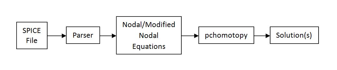
is therefore implemented through the use of two software programs. First, a “Parser” [5] generates the mathematical equations from a description of the circuit
in the commonly used SPICE format. The “Parser” is a C++ program that accepts a SPICE input file and produces either nodal analysis or modified nodal analysis circuit equations
as well as their Jacobian matrices. These equations could then be solved using homotopy methods. The MATLAB algorithm “pchomotopy” calculates the solutions. This algorithm uses
the predictor-corrector method to solve the differential equation which describes the homotopy path. A script file called “Main.m” implements the algorithm and plots the
homotopy paths.
[Top] Homotopy function used
Various homotopies may be constructed from the circuit’s nodal
or modified nodal formulations.
The fixed-point homotopy used is based on the equation
H(x, λ) = (1 - λ)G(x - a) + λF(x), (10)
where, in addition to the parameter λ, a random vector a also known as starting vector and a new parameter (a diagonal scaling matrix) G ∈ Rn × Rn are embedded.
[Top] Examples
Implementation of homotopy algorithms need not necessarily rely on large numerical
solvers or proprietary circuit simulation tools. MATLAB implementation was successfully used to find three DC operating points of the Schmitt Trigger circuit and nine DC operating
points of a benchmark four-transistor circuit. Parser was used to generate nodal analysis and modified nodal analysis equations. Even though Newton-Raphson method solvers like
PSPICE and SPICE3F5 will calculate only one DC operating point, it is possible to give PSPICE an initial guess that is close to a desired solution by using the .NODESET option.
In this manner, by using the MATLAB results as a starting point, we have found all DC operating points. The operating points calculated by MATLAB are consistent with the results
calculated by a commonly used circuit simulator PSPICE.
[Top] Ebers-Moll transistor model
Bipolar-junction transistors are modelled using the Ebers-Moll
transistor model [7]
(11)
(12)
where
and
(13)
and the reciprocity condition holds:
(14)
For npn transistors: me < 0, mc < 0, and n < 0.
For pnp transistors: me > 0, mc > 0, and n > 0.
[Top] Schmitt Trigger circuit no. 1
The application of homotopy methods is illustrated by solving non-linear equations that describe the Schmitt Trigger circuit shown in Fig. 1. The circuit possesses three DC operating points. All three solutions to the circuit’s nodal equations and modified nodal equations were successfully found by using the fixed-point homotopy (10).
[Top] Circuit Diagram :
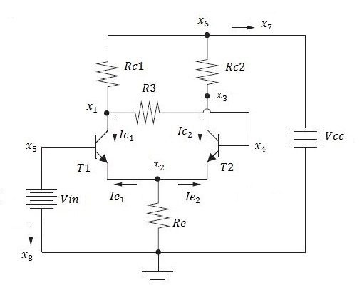
Fig. 1. Schmitt Trigger circuit whose equations were solved by using homotopy method. Circuit parameters: R3 = 10 kΩ, Rc1 = 2 kΩ, Rc2 = 1 kΩ, Re = 100 Ω, Vcc = 10 V and Vin = 1.5 V. The two bipolar transistors are identical with parameters: meaf = mcar = Is = - 1.0 x 10⁻¹⁶ A, af = 0.99, ar = 0.5 and n = -38.78 1/V.
From the circuit:
(15)
where,
(16)
[Top] Nodal Equations :
(17)
[Top] Modified Nodal Equations :
(18)
[Top] Results :
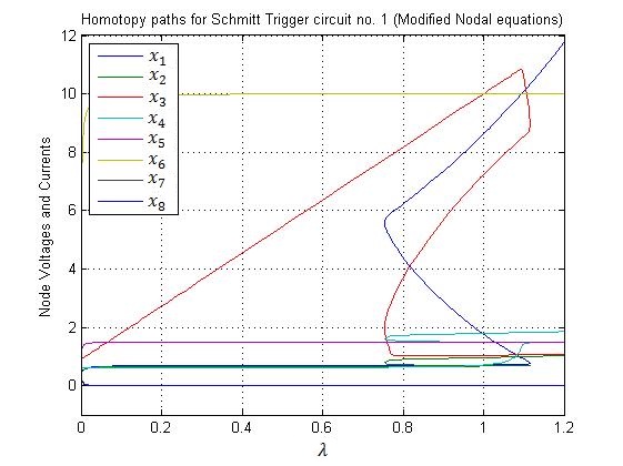
Fig. 2. Homotopy paths for the six node voltages x1 through x6 and the two currents x7 and x8 of the Schmitt Trigger circuit shown in Fig. 1. The plot shows solutions of the homotopy equations vs. the value of the homotopy parameter λ.
[Top] Solutions :
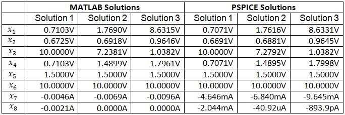
Table I. Three solutions were found by solving the circuit’s modified nodal equations using the fixed-point homotopy as well as the PSPICE simulator. Variables x1 through x6 are node voltages and variables x7 and x8 are the currents flowing through the independent voltage sources Vcc and Vin respectively.
[Top] Comments :
All three solutions to system of equations (17) and (18) were found successfully by using the fixed-point homotopy (10). The elements of the diagonal matrix G were set to 10-3 and the starting vector a was chosen by a random number generator. The solution paths for voltages and the currents as functions of the homotopy parameter λ are shown in Fig. 2. These paths were obtained by solving circuit’s modified nodal equations with a simple homotopy embedding (10). The solutions are obtained when these homotopy paths intersect the vertical line corresponding to λ = 1. The solutions for the circuit’s node voltages and the currents flowing through the independent voltage sources, found by using the fixed-point homotopy and PSPICE simulator are listed in Table I and are found to be in close agreement with each other.
[Top] Downloads :
MATLAB Code (Nodal Analysis)
MATLAB Code (Modified Nodal Analysis)
PSPICE Netlist
[Top] Schmitt Trigger circuit no. 2
The application of homotopy methods is illustrated by solving non-linear equations that describe the Schmitt Trigger circuit shown in Fig. 3. The circuit possesses three DC operating points. All three solutions to the circuit’s nodal equations and modified nodal equations were successfully found by using the fixed-point homotopy (10).
[Top] Circuit Diagram :
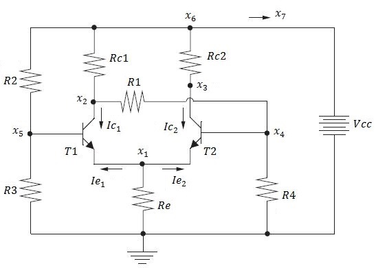
Fig. 3. Schmitt Trigger circuit whose equations were solved by using homotopy method. Circuit parameters: R1 = 10 kΩ, R2 = 5 kΩ, R3 = 1.25 kΩ, R4 = 1 MΩ, Rc1 = 1.5 kΩ, Rc2 = 1 kΩ, Re = 100 Ω and Vcc = 10 V. The two bipolar transistors are identical with parameters: meaf = mcar = Is = - 1.0 x 10⁻¹⁶ A, af = 0.99, ar = 0.5 and n = -38.78 1/V.
From the circuit:
(19)
where,
(20)
[Top] Nodal Equations :
(21)
[Top] Modified Nodal Equations :
(22)
[Top] Results :
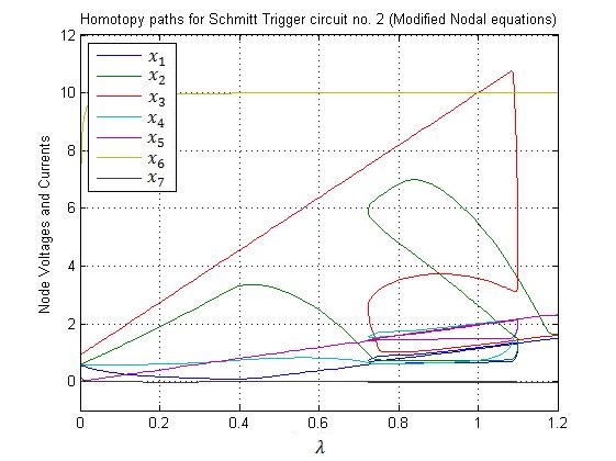
Fig. 4. Homotopy paths for the six node voltages x1 through x6 and the current x7 of the Schmitt Trigger circuit shown in Fig. 3. The plot shows solutions of the homotopy equations vs. the value of the homotopy parameter λ.
[Top] Solutions :
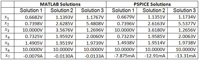
Table II. Three solutions were found by solving the circuit’s modified nodal equations using the fixed-point homotopy as well as the PSPICE simulator. Variables x1 through x6 are node voltages and variable x7 is the current flowing through the independent voltage source Vcc .
[Top] Comments :
All three solutions to system of equations (21) and (22) were found successfully by using the fixed-point homotopy (10). The elements of the diagonal matrix G were set to 10-3 and the starting vector a was chosen by a random number generator. The solution paths for voltages and the current as functions of the homotopy parameter λ are shown in Fig. 4. These paths were obtained by solving circuit’s modified nodal equations with a simple homotopy embedding (10). The solutions are obtained when these homotopy paths intersect the vertical line corresponding to λ = 1. The solutions for the circuit’s node voltages and the current flowing through the independent voltage source, found by using the fixed-point homotopy and PSPICE simulator are listed in Table II and are found to be in close agreement with each other.
[Top] Downloads :
MATLAB Code (Nodal Analysis)
MATLAB Code (Modified Nodal Analysis)
PSPICE Netlist
[Top] Chua circuit
Nine DC operating points of the four-transistor benchmark circuit shown in Fig. 5 were found by using the MATLAB implementation of the homotopy algorithm.
[Top] Circuit Diagram :
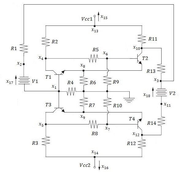
Fig. 5. Four-transistor benchmark circuit that possesses nine DC operating points. Circuit parameters: R1 = 10 kΩ, R2 = R3 = 4 kΩ, R4 = 5 kΩ, R5 = R8 = 30 kΩ, R6 = R7 = 0.5 kΩ, R9 = R10 = 10.1 kΩ, R11 = R12 = 4 kΩ, R13 = R14 = 30 kΩ, V1 = 10 V, V2 = 2 V, Vcc1 = 12 V and Vcc2 = 12 V. The four bipolar transistors are identical with parameters : meaf = mcar = Is = - 1.0 x 10⁻⁹ A, af = 0.99, ar = 0.5 and n = -38.7766 1/V.
From the circuit:
(23)
where,
(24)
[Top] Modified Nodal Equations :
(25)
[Top] Results :
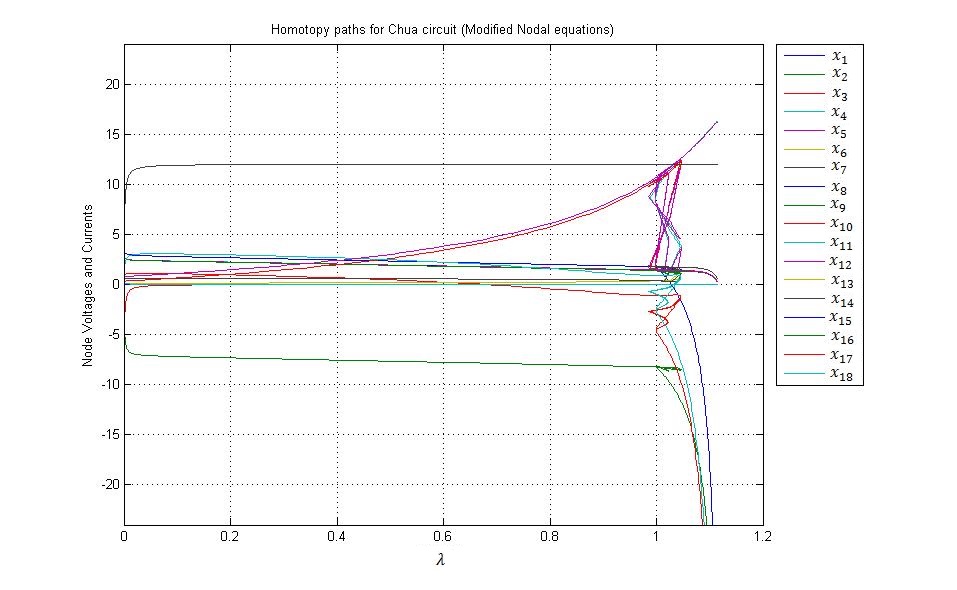
Fig. 6. Homotopy paths for the fourteen node voltages x1 through x14 and the four currents x15 through x18 flowing through the four independent voltage sources of the four transistor benchmark circuit shown in Fig. 5. The plot shows solutions of the homotopy equations vs. the value of the homotopy parameter λ.
[Top] Solutions :
Table III. Nine solutions were found by solving the circuit’s modified nodal equations using the fixed-point homotopy. Variables x1 through x14 are node voltages and variables x15 through x18 are the currents flowing through the independent voltage sources Vcc1, Vcc2, V1 and V2 respectively.
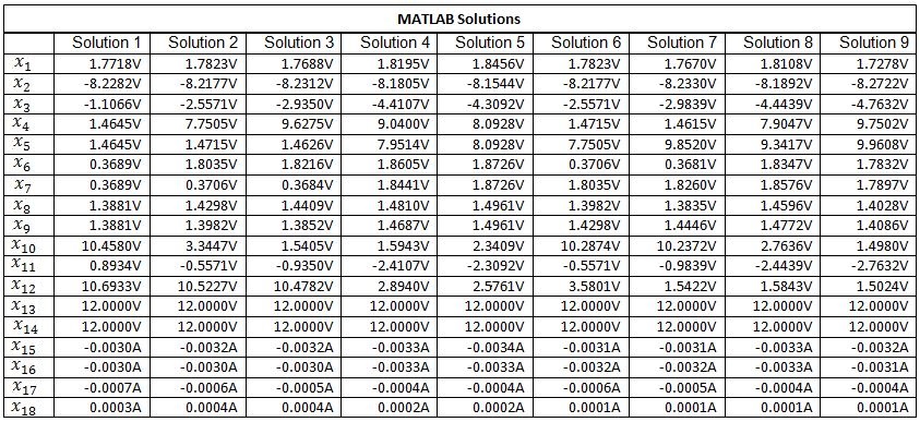
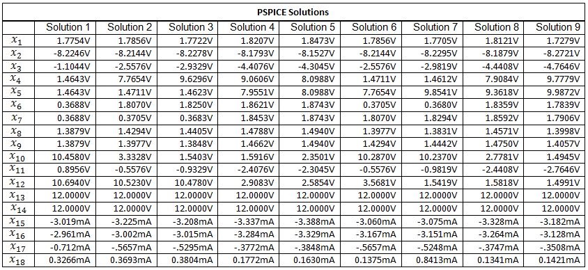
Table IV. Nine solutions each found by using PSPICE. Variables x1 through x14 are node voltages and variables x15 through x18 are the currents flowing through the independent voltage sources Vcc1, Vcc2, V1 and V2 respectively.
[Top] Comments :
All nine solutions to system of equations (25) were found successfully by using the fixed-point homotopy (10). The elements of the diagonal matrix G were set to 10-3 and the starting vector a was chosen by a random number generator. The solution paths for voltages and the current as functions of the homotopy parameter λ are shown in Fig. 6. These paths were obtained by solving circuit’s modified nodal equations with a simple homotopy embedding (10). The solutions are obtained when these homotopy paths intersect the vertical line corresponding to λ = 1. The solutions for the circuit’s node voltages and the current flowing through the independent voltage source, found by using the fixed-point homotopy and PSPICE simulator are listed in Table III and Table IV respectively and are found to be in close agreement with each other.
[Top] Downloads :
MATLAB Code (Modified Nodal Analysis)
PSPICE Netlist
[Top] References
[1] Lj. Trajkovic, “DC Operating points of transistor circuits,” Nonlinear Theory and Its Applications,
IEICE, vol. 3, no. 3, pp. 287-300, July 2012.
[2] A. Dyess, E. Chan, H. Hofmann, W. Horia and Lj. Trajkovic, “Simple implementations of homotopy algorithms for
finding dc solutions of nonlinear circuits,” in Proc. IEEE Int. Symp. Circuits and Systems, Orlando, FL, vol. 6, pp. 290-293, June 1999.
[3] K. Yamamura, T. Sekiguchi, and Y. Inoue, “A fixed-point homotopy method for solving modified nodal equations,” IEEE Trans. Circuits Syst. I, vol. 46, no. 6,
pp. 654–664, June 1999.
[4] W. Horia, “New Numerical Algorithms for Simulating Electronic Circuit,” URO Report, EECS Department, UC Berkeley, May 1997.
[5] E. Chan, “PARSER: a program for writing nodal and modified nodal analysis equations from a SPICE-like circuit description,” URO Report, EECS Department, UC Berkeley, December
1996.
[6] H. Hofmann, “EECS 290N: Final Project Report,” EECS Department, UC Berkely, May 1996.
[7] J. J. Ebers and J. L. Moll, “Large scale behavior of junction transistors,” in Proc. of IRE, pp. 1761–1772, December 1954.
[Top] About Archit
 Archit Singhal is an undergraduate student at Indian Institute of Technology Roorkee, India.
He is a final year student pursuing his bachelors with Electrical Engineering major (2010-2014).
This work was done as a part of his summer internship (May-July 2013) under
MITACS Globalink Program with professor Ljiljana Trajkovic at
Simon Fraser University guided by Deepali Arora from
University of Victoria.
Please email questions or bug reports related to this work to him at singhalarchit1@gmail.com.