4. Two Real Poles

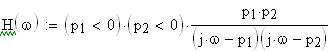
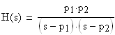
Now back to lowpass behaviour. There are plenty of systems with more than one time constant, so you will run across this form many times. I have to admit it's not very exciting, but the animation will at least demonstrate a point in modelling of systems. This tranfer function is set up for unit gain at DC:

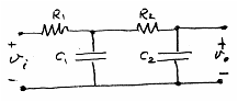
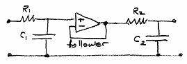
Here are a couple of circuits that are described by a transfer function of this form. Note that the poles of the left hand circuit are not -1/R₁C₁ and -1/R₂C₂, the poles of the two sections individually, because the second section loads the first (i.e., drains current from it), thereby shifting the pole location. However, if you really, really want the transfer function to be the product of the section transfer functions and you can afford an op amp, then the right hand circuit will do it.

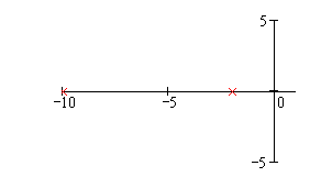
For the animation, we'll start with a large negative value of one of the poles and sweep it in to the origin, leaving the other one fixed. The pole doesn't go into the right half plane, even though unstable systems still have step and impulse responses. The image below is a scene from the animation. Click here to view the animation and leave the animation window open as you read this section. Drag the animation slider back and forth with your mouse to get different parameter values and change all the graphs together.

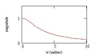
As usual, time constants are negative reciprocals of the pole locations (e.g., t₁ = -1/p₁), if the poles are real. The bandwidth decreases and the changing time constant becomes longer as the moving pole gets closer to the origin. Note the inverse relationship between the bandwidth of the frequency response and the width of the impulse response.

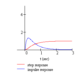
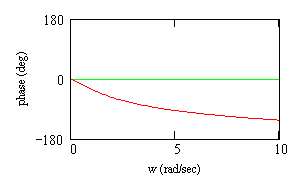
Compare these with the plots for the single time constant sytem . The impulse response here is smeared out with a second time constant, so it doesn't have a jump discontinuity at time zero like the STC system. The phase shift starts at zero here, just as it does in the STC system, but it has a final value of -180 degrees, not -90, again because of the second pole.

Now for that point of modelling. When one of the poles is much farther out than the other, its time constant is much shorter than that of the other pole. The resulting impulse and step responses look remarkably like those of the single time constant (STC) system you saw in Section 1 . Consequently, you could approximate this system by the single time constant system, at least for input signals that have temporal fine structure that is much longer than the shorter of the system's time constants. Equivalently, for input signals with bandwidth that is much less than the location of the farther pole. The model won't be perfect, but it may be good enough for quick reasoning. As for the ultimate 180 degree phase shift here, compared with 90 degrees for the STC system, it won't show up much over the bandwidth of the signal, which is assumed to be much smaller than that of the outer pole, so perhaps you don't care.

This type of system is an easy way to get a lowpass characteristic to smooth out the noise in a signal. You can use resistors and capacitors alone, without inductors. On the other hand, its frequency response sags even for small frequencies, so it also distorts any desired (i.e., non-noise) component of the signal.

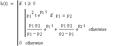
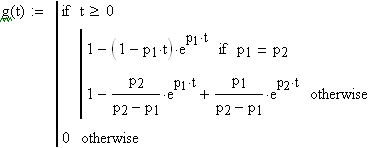
In defining the impulse and step responses, we have to allow for the possibility that p₁=p₂, since a double pole produces a different functional form of the solution, one that sidesteps the division by zero that would result from use of the standard form. Both of these expressions were obtained by performing an inverse Laplace transform.