6. TWO COMPLEX POLES - THE LOWPASS FORM
About This System
Systems with complex poles can have oscillations in their impulse and step responses, which makes them very useful in filter design.
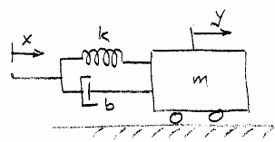
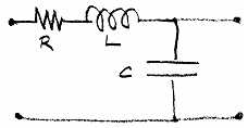
This section highlights second order systems with complex poles and no zeros. The absence of zeros allows a non-zero steady state response to a step input. The sketches below show a couple of systems that are described by such a transfer function. They both have more than one form of energy storage (capacitive and inductive, spring and mass), which is a characteristic feature of passive systems with complex poles. In the mechanical system, the output is displacement of the mass in response to displacement of the spring/damper assembly. They both have a non-zero steady state response to a step input.
If they are lightly damped (i.e., little power lost in the dissipative elements compared with power flow in the storage elements), then these systems can resonate. The animations will show this behaviour. However, if such systems are part of a design, rather than something provided by nature, then it is more common not to make them strongly resonant. Instead, we use the fact of non-zero DC gain, and set them up just slightly underdamped, in order to make a good lowpass filter.
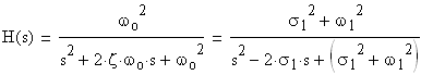
Any second order lowpass transfer function looks like this when normalized for unit gain at DC (s = 0):
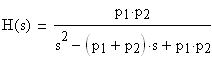
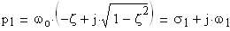
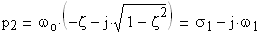
where p1 and p2 are the two poles and there are no zeros. Since complex poles occur in conjugate pairs, we can characterize them by two real parameters, such as the real and imaginary parts of one of them. We will use two common ways to describe the pole locations: natural frequency wo & damping factor z, and real part s1 & imaginary part w1. We are interested in complex poles, so they look like this:
pole nat freq & damp. fact. re and im parts
and the transfer function is then written, in two forms, as
The poles are complex for z < 1 (underdamped) and real for z > 1 (overdamped). The case z = 1 is termed critically damped. The system is stable for s1 < 0.
We'll see two set of animations: one set for the wo, z parameterization and one for the s1, w1 parameterization. In each case, we'll hold one of the variables constant and sweep the other.
Animated Responses
Damping Factor and Natural Frequency
Sweep z
First, fix the natural frequency wo at 1 rad/sec and sweep the damping factor z from a positive value down to zero (we won't bother with negative values, which give unstable systems). Click
here
to see the animation and leave the animation window open as you read this section. Drag the slider back and forth with your mouse to get different parameter values. You can see that, for complex poles, wo is the pole radius (constant at 1) and z is the sine of the angle between the pole and the imaginary axis.
When the poles are real (z > 1), we have the system with two real poles that we investigated in
Section 4
, so there is nothing new. When they start to move out on the circle (complex poles), it gets more interesting, as oscillations show up in the time responses, and resonance can be seen in the frequency responses. The time constant is the negative reciprocal of the real part of the pole locations (t = -1/(zwo)) and the oscillation frequency (the damped natural frequency) is the imaginary part of the pole locations (wd = sqrt(1-z2)wo). Evidently, z controls the overall shape of the response.
Set z to be 0.707 (= 1/sqrt(2)), to make the radial line at 45 degrees. This gives a special type of system response, discussed further below under Uses.
For small values of z, there are many oscillations in the time response. This condition is termed resonance, and the number of oscillations per time constant is determined solely by z. In resonant conditions, the interesting action in the frequency responses (both magnitude and phase) is confined to a narrow region around the resonant frequency. The oscillation frequency (the damped natural frequency wd) approaches the natural frequency wo.
Sweep wo
Next, fix the damping factor z at 0.25 and sweep the natural frequency wo from 0.1 out to 1.4 rad/sec. Click
here
to see the animation, and drag the slider back and forth with your mouse to get different parameter values. You can see that, as the pole radius wo increases, the poles move out along a radial line with angle determined by z (the sine of the angle between the pole and the imaginary axis).
Unlike z, the natural frequency wo does not affect the general shape of the responses. Instead, it acts as a time-frequency scale factor. Increasing wo expands the scale of the frequency response and of the pole-zero diagram (which is also in the frequency domain). The increase of wo also compresses the time scale of the step and impulse responses.
Real and Imaginary Parts
Sweep s1
First, we will fix the imaginary part w1 of the first conjugate pole at 1 rad/sec and sweep the real part s1 from a negative value in to the origin. Click
here
to see the animated responses and leave the animation window open as you read this section. Drag the slider back and forth with your mouse to get different parameter values.
Since the time constant is the negative reciprocal of the real part of the poles (t = -1/s1), we see that the effect of changing s1 with a constant w1 is simply to change the time constant. The oscillation frequency (the damped natural frequency wd, which also equals w1) remains constant.
Sweep w1
Finally, we fix the real part s1 of the poles to -0.25 sec-1 and sweep the imaginary part w1 from 0.2 rad/sec out to 3 rad/sec. Click
here
to see the result. Drag the slider back and forth with your mouse to get different parameter values.
In the step and impulse responses, you see that the time constant t does not change (why?), but the oscillation frequency wd (the damped natural frequency) increases (again, why?).
In the frequency response, you see that the centre frequency increases. However, the bandwidth (which is about 1/(2t)) stays constant, so the changes in amplitude and phase take place over the same range of frequencies, just with a different centre..
Uses
This filter has non-zero DC gain, since it has no zeros. Despite the possibility of resonant behaviour, it is not normally used as a bandpass filter. Instead, it is widely used as a lowpass filter when z = 1/sqrt(2) = 0.707. You can see why in the animation if you drag the slider to get z close to 0.707. In the time domain, its step response has a fast rise time with a level of overshoot that is acceptable for most purposes. In the frequency domain, it is "maximally flat"; that is, the magnitude of the frequency response sags very slowly (zero derivatives at DC) with increasing frequency up to the corner frequency. Similarly, the phase shift is almost linear up to the same point. Together, they mean less distortion of a low frequency desired signal and more suppression of unwanted higher frequencies than in the simple one pole lowpass of
Section 2
.
The filter with z = 0.707 is known as a "second order Butterworth" filter. Higher order Butterworth filters - flatter in-band and with a faster dropoff in frequency out of band - are generated by placing several poles in an equispaced manner around the left half of the circle.
This type of response is useful in mechanical systems, too. Remember the sketched mechanical system at the top of the page? It can represent a mechanical system with a spring and shock absorbers.
We don't always choose z = 0.707. In electronic and mechanical systems, it is sometimes important not to have overshoot in the response to a step input. Yet it is also important to have a fast response, rather than a sluggish one. A critically damped system - in which the two real poles are equal - equivalently, z = 1 - gives the shortest rise time without overshoot.
Try it
in the animation.
===================================================================
Work Area
The work area, in which the animations are prepared, is quite large for this worksheet. If you want to have a look at it, click
here
.
.