7. TWO COMPLEX POLES - THE RESONANT BANDPASS FILTER
About This System
Finally, two complex poles and a zero. This is the bandpass form. With light damping, it becomes resonant, and is widely used to extract tones or other narrowband signals from noise. Its selectivity is MUCH greater than that of the bandpass circuit with two real poles and a zero that you saw in
Section 5
.
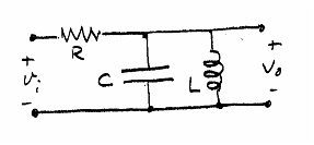
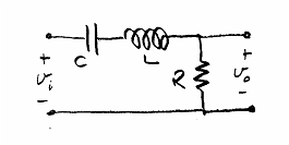
The sketches below show a few systems that are described by such a transfer function. The series RLC and the RLC "tank" circuit should be familiar to you.
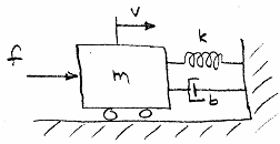
This mechanical system has velocity of the cart as output in response to the applied force.
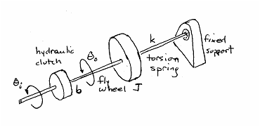
The hydraulic clutch couples its input and output shafts through a viscous fluid. The torsional spring provides torque proportional to the angular difference of its two ends.
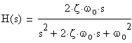
Systems with complex poles can show oscillatory behaviour, including resonance. Since poles occur in conjugate pairs, we can characterize them by two real parameters, such as the real and imaginary parts of one of them. We'll use an alternative parameterization, though, with the natural frequency wo and the damping factor z. The transfer function looks like this when normalized for unit gain at resonance:
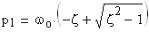
Its poles
are real for z>1 (overdamped) and complex for z<1 (underdamped). The case z=1 is termed critically damped. In this bandpass form, we're usually interested in extreme underdamping, where z is very small.
Animated Responses
We'll see two animations: one for changing the damping factor z and one for changing the natural frequency wo. Animations for the alternative parameterization (with real and imaginary parts), are omitted in this section, because the main points to be gained from them were illustrated in
Section 5
, on the lowpass form.
Sweep z
To see the range of responses, we'll sweep the damping factor z from unity down to zero (we won't bother with negative values, which give unstable systems, or with values greater than 1, which we examined in
Section 5
). We'll normalize the natural frequency wo to 1. Click
here
to see the animated response and keep the animation window open as you read this section. Drag the slider back and forth in the animation to get different parameter values.
When the poles approach the imaginary axis, we see strong resonance, and the interesting action in the frequency responses (both magnitude and phase) is confined to an increrasingly narrow region around the resonant frequency. The resonant frequency (i.e., maximum response) is the natural frequency wo.
As z becomes small, the poles move more or less horizontally as they approach the imaginary axis. In this region, the time responses (step, impulse responses) show a constant oscillation frequency (the damped natural frequency wd is almost equal to the natural frequency wo) and an increasing time constant.
The step and impulse responses both become smaller near resonance because our formulation of the transfer function was normalized for unit gain at resonance. In more detail... as you saw in the
animation of convolution
, the impulse response of a resonant filter contains many oscillations in a time constant, so that the convolution with an input sine wave at the resonant frequency produces many half-cycles of a consistent sign, positive or negative; consequently, they amplitude of those half-cycles doesn't have to be large, which means the impulse response amplitude does not have to be large. An alternative explanation is that the narrow passband of the filter only admits a small amount of the total energy in the step or impulse input, which is spread over a wide range of frequencies.
Remember, though, that our normalization to unit gain at resonance was for convenience. A resonant mechanical or electrical system may have some other gain; its output amplitude may be much greater than the input amplitude.
Sweep wo
Next, fix the damping factor z at 0.25 and sweep the natural frequency wo from 0.1 out to 1.4 rad/sec. Click
here
to see the animation, and keep the animation window open as you read this section. Drag the slider back and forth with your mouse to get different parameter values. You can see that, as the pole radius wo increases, the poles move out along a radial line with angle determined by z (the sine of the angle between the pole and the imaginary axis).
Unlike z, the natural frequency wo does not affect the time constant. Instead, it acts as a time-frequency scale factor. Increasing wo expands the scale of the frequency response and of the pole-zero diagram (which is also in the frequency domain). The increase of wo also compresses the time scale of the step and impulse responses.
Uses
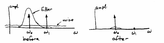
This resonant bandpass filter is commonly used to extract a tone or other narrowband signal from wideband noise. A bank of such filters, each tuned to a different frequency, provides a detector for a tone-coded control system (a different tone for each action desired of the remote station).
======================================================
Work Area
The work area for this one is rather large, so it's in a
separate file
.
.