CTM Example: DC Motor Speed Modeling

Example: DC Motor Speed Modeling

Physical setup and system equations
Design requirements
Matlab representation and open-loop response

Physical setup and system equations

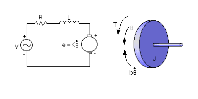
Photo courtesy: Pope Electric Motors Pty Limited

A common actuator in control systems is the DC motor. It directly provides rotary motion and, coupled with wheels or drums and cables, can provide transitional motion. The electric circuit of the armature and the free body diagram of the rotor are shown in the following figure:

For this example, we will assume the following values for the physical parameters. These values were derived by experiment from an actual motor in Carnegie Mellon's undergraduate controls lab.

* moment of inertia of the rotor (J) = 0.01 kg.m^2/s^2
* damping ratio of the mechanical system (b) = 0.1 Nms
* electromotive force constant (K=Ke=Kt) = 0.01 Nm/Amp
* electric resistance (R) = 1 ohm
* electric inductance (L) = 0.5 H
* input (V): Source Voltage
* output (theta): position of shaft
* The rotor and shaft are assumed to be rigid

The motor torque, T, is related to the armature current, i, by a constant factor Kt. The back emf, e, is related to the rotational velocity by the following equations:

In SI units (which we will use), Kt (armature constant) is equal to Ke (motor constant).

From the figure above we can write the following equations based on Newton's law combined with Kirchhoff's law:

1. Transfer Function

Using Laplace Transforms, the above modeling equations can be expressed in terms of s.

By eliminating I(s) we can get the following open-loop transfer function, where the rotational speed is the output and the voltage is the input.

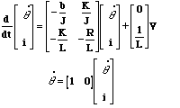
2. State-Space

In the state-space form, the equations above can be expressed by choosing the rotational speed and electric current as the state variables and the voltage as an input. The output is chosen to be the rotational speed.

Design requirements

First, our uncompensated motor can only rotate at 0.1 rad/sec with an input voltage of 1 Volt (this will be demonstrated later when the open-loop response is simulated). Since the most basic requirement of a motor is that it should rotate at the desired speed, the steady-state error of the motor speed should be less than 1%. The other performance requirement is that the motor must accelerate to its steady-state speed as soon as it turns on. In this case, we want it to have a settling time of 2 seconds. Since a speed faster than the reference may damage the equipment, we want to have an overshoot of less than 5%.

If we simulate the reference input (r) by an unit step input, then the motor speed output should have:

Settling time less than 2 seconds
Overshoot less than 5%
Steady-state error less than 1%

Matlab representation and open-loop response

1. Transfer Function

We can represent the above transfer function into Matlab by defining the numerator and denominator matrices as follows:

Create a new m-file and enter the following commands:

J=0.01;
b=0.1;
K=0.01;
R=1;
L=0.5;
num=K;
den=[(J*L) ((J*R)+(L*b)) ((b*R)+K^2)];

Now let's see how the original open-loop system performs. Add the following commands onto the end of the m-file and run it in the Matlab command window:

step(num,den,0:0.1:3)
title('Step Response for the Open Loop System')

You should get the following plot:

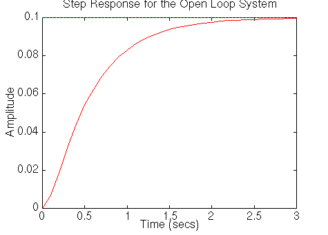
From the plot we see that when 1 volt is applied to the system, the motor can only achieve a maximum speed of 0.1 rad/sec, ten times smaller than our desired speed. Also, it takes the motor 3 seconds to reach its steady-state speed; this does not satisfy our 2 seconds settling time criterion.

2. State-Space

We can also represent the system using the state-space equations. Try the following commands in a new m-file.

J=0.01;
b=0.1;
K=0.01;
R=1;
L=0.5;
A=[-b/J   K/J
   -K/L   -R/L];
B=[0
   1/L];
C=[1   0];
D=0;

step(A, B, C, D)

Run this m-file in the Matlab command window, and you should get the same output as the one shown above.

User feedback

Modeling Examples: Cruise Control | Motor Speed | Motor Position | Bus Suspension | Inverted Pendulum | Pitch Controller | Ball and Beam
Motor Speed Examples: Modeling | PID | Root Locus | Frequency Response | State Space | Digital Control: PID
Tutorials: Basics | Modeling | PID | Root Locus | Frequency Response | State Space | Digital Control | Examples

8/7/97 BRN
8/24/97 WM