

|
|
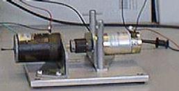 A common actuator in control systems is the DC motor. It directly
provides rotary motion and, coupled with wheels or drums and cables,
can provide transitional motion. The electric circuit of the armature
and the free body diagram of the rotor are shown in the following
figure:
For this example, we will assume the following values for the physical parameters. These values were derived by experiment from an actual motor in Carnegie Mellon's undergraduate controls lab.
In SI units (which we will use), Kt (armature constant) is equal to Ke (motor constant).
From the figure above we can write the following equations based on Newton's law combined with Kirchhoff's law:
By eliminating I(s) we can get the following transfer function, where the rotating speed is the output and the voltage is an input.
However during this example we will be looking at the position, as being the output. We can obtain the position by integrating Theta Dot, therefore we just need to divide the transfer function by s.
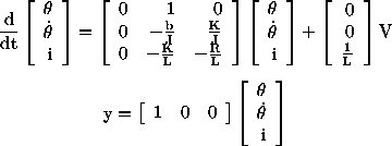
We will want to be able to position the motor very precisely, thus the steady-state error of the motor position should be zero. We will also want the steady-state error due to a disturbance, to be zero as well. The other performance requirement is that the motor reaches its final position very quickly. In this case, we want it to have a settling time of 40ms. We also want to have an overshoot smaller than 16%.
If we simulate the reference input (R) by a unit step input, then the motor speed output should have:
Create a new m-file and enter the following commands:
J=3.2284E-6;
b=3.5077E-6;
K=0.0274;
R=4;
L=2.75E-6;
num=K;
den=[(J*L) ((J*R)+(L*b)) ((b*R)+K^2) 0];
Now let's see how the original open-loop system performs. Add the following command onto the end of the m-file and run it in the Matlab command window:
step(num,den,0:0.001:0.2)You should get the following plot:
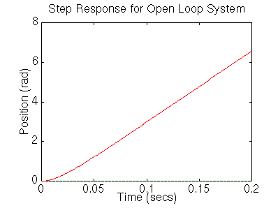
From the plot we see that when 1 volt is applied to the system, the motor position changes by 6 radians, six times greater than our desired position. For a 1 volt step input the motor should spin through 1 radian. Also, the motor doesn't reach a steady state which does not satisfy our design criteria
J=3.2284E-6;
b=3.5077E-6;
K=0.0274;
R=4;
L=2.75E-6;

A=[0 1 0
   0 -b/J K/J
   0 -K/L -R/L];
B=[0 ; 0 ; 1/L];
C=[1 0 0];
D=[0];
The step response is obtained using the command
step(A,B,C,D)
Unfortunately, Matlab responds with
Warning: Divide by zero
???  Index exceeds matrix dimensions.

Error in ==> /usr/local/lib/matlab/toolbox/control/step.m
On line 84  ==> dt = t(2)-t(1);
There are numerical scaling problems with this representation of the dynamic equations. To fix the problem, we scale
time by tscale = 1000. Now the output time will be in milliseconds rather than in seconds.
The equations are given by
tscale = 1000;
J=3.2284E-6*tscale^2;
b=3.5077E-6*tscale;
K=0.0274*tscale;
R=4*tscale;
L=2.75E-6*tscale^2;

A=[0 1 0
   0 -b/J K/J
   0 -K/L -R/L];
B=[0 ; 0 ; 1/L];
C=[1 0 0];
D=[0];
The output appears the same as when obtained through the transfer function, but the time vector must be divided by tscale.
[y,x,t]=step(A,B,C,D);
plot(t/tscale,y)
ylabel('Amplitude')
xlabel('Time (sec)')