
|
|
Open-loop poles
LQR design
Adding the reference Input
Observer design
The state equations for this problem are:
The design criteria for this system with the cart receiving a 0.2 m step input are as follows:
To see how this problem was originally set up, consult the inverted pendulum modeling page.
This problem can be solved using full state feedback. The schematic of this type of control system is shown below:
If you are interested in running an animation of this example based on the control techniques used in the state-space tutorial please go to the Inverted Pendulum Animation Page after completing this tutorial.
In this problem R represents the commanded step input to the cart. The 4 states represent the position and velocity of the cart and the angle and angular velocity of the pendulum. The output y contains both the position of the cart and the angle of the pendulum. We want to design a controller so that when an step input is given to the system, the pendulum should be displaced, but eventually return to zero (i.e. the vertical) and the cart should move to it's new commanded position. To view the system's open-loop response please refer to the inverted pendulum modeling Page
The first step in designing this type of controller is to determine the open-loop poles of the system. Enter the following lines of code into a m-file (or a '.m' file located in the same directory as Matlab):
     M = 0.5;
     m = 0.2;
     b = 0.1;
     i = 0.006;
     g = 9.8;
     l = 0.3;

     p = i*(M+m)+M*m*l^2; %denominator
     A = [0      1             0        0;
	           0 -(i+m*l^2)*b/p (m^2*g*l^2)/p  0;
	           0      0             0        1;
	           0 -(m*l*b)/p    m*g*l*(M+m)/p 0];
     B = [0; (i+m*l^2)/p; 0; m*l/p];
     C = [1 0 0 0;
          0 0 1 0];
     D = [0;0];

     p = eig(A)
The Matlab command window should output the following text as a result:
The next step in the design process is to assume that we have full-state feedback (i.e. that we can measure all four states), and find the vector K which determines the feedback control law. This can be done in a number of ways. If you know the desired closed-loop poles, you can use the place or acker command. Another option is to use the lqr function; this will give you the optimal controller (under certain assumptions; consult your textbook for more details). The lqr function allows you to choose two parameters, R and Q, which will balance the relative importance of the input and state in the cost function that you are trying to optimize. The simplest case is to assume R=1, and Q=C'*C. You may notice that we are using both outputs (the pendulum's angle and the cart's position). Essentially, the lqr method allows for the control of both outputs. In this case, it is pretty easy to do. The controller can be tuned by changing the nonzero elements in the Q matrix to get a desirable response.
To find the structure of Q, enter the following into the Matlab command window:
The curve in green represents the pendulum's angle, in radians and the curve in blue represents the cart's position in meters. As you can see, this plot is not satisfactory. The pendulum and cart's overshoot appear fine, but their settling times need improvement and the cart's rise time needs to go down. As I'm sure you have noticed the cart is not near the desired location but has in fact moved in the other direction. This error will be dealt with in the next section and right now we will focus on the settling and rise times. Go back to your m-file and change the x and y variables to see if you can get a better response. You will find that increasing x makes the settling and rise times go down, and lowers the angle the pendulum moves. Using x=5000 and y=100, the following value of K and step response were found:
You may have noted that if you increased x and y even higher, you could improve the response even more. The reason this plot was chosen was because it satisfied the design requirements while keeping x and y as small as possible. In this problem, x and y have been used to describe the relative weight of the tracking error in the cart's position and pendulum's angle versus the control effort. The higher x and y are, the more control effort is used, but the smaller the tracking error. The system response has a settling time under 2 seconds.
Now we want to get rid of the steady-state error. In contrast to the other design methods, where we feedback the output and compare it to the reference input to compute an error, with a full-state feedback controller we are feeding back all the states. We need to compute what the steady-state value of the states should be, multiply that by the chosen gain K, and use a new value as our reference for computing the input. This can be done by adding a constant gain Nbar after the reference. The schematic below shows this relationship:
Nbar can be found using the user-defined function rscale (copy it to the directory that your m-file is in). Delete the lsim line and copy the following to your m-file and run it to view the step response with Nbar added.
A different C had to be used because the rscale function will not work for multiple outputs. However, the Nbar found is correct, as you can see from the output below:
Now, the steady-state error is within our limits, the rise and settling times are met and the pendulum's overshoot is within range of the design criteria.
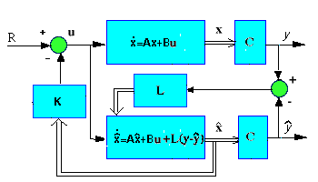
This response is good, but was found assuming full-state feedback, which most likely will not be a valid assumption. To compensate for this, we will next design a full-order estimator to estimate those states that are not measured. A schematic of this kind of system is shown below, without Nbar:

To begin, we must first find the controller poles. To do this copy the following code to the end of your m-file:
You should see the following in the Matlab window:
This response is about the same as before. All of the design requirements have been met with the minimum amount of control effort, so no more iteration is needed.
As you can see, it is much easier to control multi-input or multi-output systems with the state space method than with any other of the methods.
If you are interested in running an animation of the inverted pendulum example based on the control techniques used in this tutorial please go to the Inverted Pendulum Animation Page.
Tutorials