
|
|
Adding a PID controller
Plotting the closed-loop response
Choosing the gains for the PID controller
From the main problem, the dynamic equations in transfer function form are the
following:


and the system schematic looks like:
For the original problem setup and the derivation of the above equations and schematic, please refer to the bus modeling page.
We want to design a feedback controller so that when the road disturbance (W) is simulated by a unit step input, the output (X1-X2) has a settling time less than 5 seconds and an overshoot less than 5%. For example, when the bus runs onto a 10 cm high step, the bus body will oscillate within a range of +/- 5 mm and will stop oscillating within 5 seconds.
The system model can be represented in Matlab by creating a new m-file and entering the following commands (refer to main problem for the details of getting those commands).
m1=2500;
m2=320;
k1 = 80000;
k2 = 500000;
b1 = 350;
b2 = 15020;

nump=[(m1+m2) b2 k2]
denp=[(m1*m2) (m1*(b1+b2))+(m2*b1) (m1*(k1+k2))+(m2*k1)+(b1*b2) (b1*k2)+(b2*k1) k1*k2]

num1=[-(m1*b2) -(m1*k2) 0 0]
den1=[(m1*m2) (m1*(b1+b2))+(m2*b1) (m1*(k1+k2))+(m2*k1)+(b1*b2) (b1*k2)+(b2*k1) k1*k2]

numf=num1;
denf=nump;
Recall that the transfer function for a PID controller is:
where KP is the proportional gain, KI is the integral gain, and KD is the derivative gain. Let's assume that we will need all three of these gains in our controller. To begin, we might start with guessing a gain for each: KP=208025, KI=832100 and KD=624075. This can be implemented into Matlab by adding the following code into your m-file:
KD=208025;
KP=832100;
KI=624075;
numc=[KD,KP,KI];
denc=[1 0];
Now let's simulate the response of the system (the distance X1-X2) to a step disturbance on the road. From the schematic above we can find the transfer function from the road disturbance W to the output(X1-X2):
numa=conv(conv(numf,nump),denc);
dena=conv(denf,polyadd(conv(denp,denc),conv(nump,numc)));
Note that the function "polyadd" is not a standard function in Matlab; you will need to copy it to a new m-file to use it. Click here for more information on defining new functions in Matlab.
Refer to the bus modeling page, nump = denf as we can see in the matlab command above. Thus we can simplified this transfer function to be the following:
numa=conv(numf,denc);
dena=polyadd(conv(denp,denc),conv(nump,numc));
Now we have created the closed-loop transfer function in Matlab that will represent the plant, the disturbance, as well as the controller. Let's see what the closed-loop step response for this system looks like before we begin the control process. Keep in mind that we are going to use a 0.1 m high step as our disturbance, to simulate this, all we need to do is to multiply numa by 0.1. Add the following code into your m-file:
t=0:0.05:5;
step(0.1*numa,dena,t)
title('closed-loop response to 0.1m high step w/ pid controller')
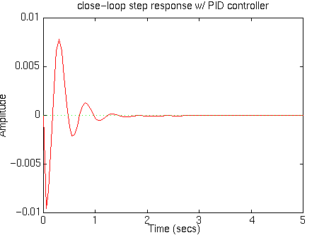
you should see the response
(X1-X2) to a step W like this:

z1=1;
z2=3;
p1=0;
numc=conv([1 z1],[1 z2])
denc=[1 p1]
num2=conv(nump,numc);
den2=conv(denp,denc);
rlocus(num2,den2)
title('root locus with PID controller')
[K,p]=rlocfind(num2,den2)
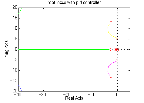
you should see the closed-loop poles and zeros on the s-plane like this and
you can choose the gain and dominant poles on the graph by yourself:

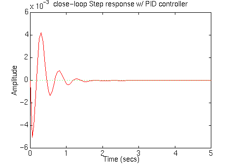
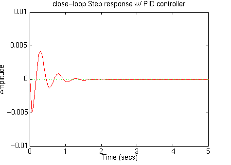
Now that we have the closed-loop transfer function, controlling the system is simply a matter of changing the KD,KP,and KI variables. From the figure above, we can see that the system has larger damping than required, but the settling time is very short. This response still doesn't satisfy the 5% overshoot requirement. As mentioned before, this can be rectified by adjusting the KD, KP and KI variables to find better response. Let's increase KP,KI,KD by 2 times to see what will happen. Go back to your m-file and multiply KP,KI,KD by 2 and then rerun the program, you should get the following plot:

To compare this graph with the graph of low-gain PID controller, you can change the axis:
axis([0 5 -.01 .01])

For this problem, it turns out that the PID design method adequately controls the system. This can been seen by looking at the root locus plot. Such a task can be achieved by simply changing only the gains of a PID controller. Feel free to play around with all three of the parameters,KD,KP and KI, as we suggested, but you will most likely get the response to have either large percent overshoot or very long settling time. But if you do find a good PID design, please email us with your results! We are always interested in different ways to solve our examples; we may include your solution in a future version of these tutorials.