Example: State Space Design for Digital Bus Suspension Control

Sampling Time Selection
Continuous to Discrete Conversion
Designing the Controller
Simulating the Closed-Loop Response

In this example, we will design a digital state space controller for the bus suspension control example. First we will convert the continuous time model to a discrete time model, and then use the pole placement method to design the controller. From the bus suspension state space modeling page, the state space model of the system is:

Where:: * body mass (m1) = 2500 kg,; * suspension mass (m2) = 320 kg,; * spring constant of suspension system(k1) = 80,000 N/m,; * spring constant of wheel and tire(k2) = 500,000 N/m,; * damping constant of suspension system(b1) = 350 Ns/m.; * damping constant of wheel and tire(b2) = 15,020 Ns/m.; * control force (u) = force from the controller we are going to design.
The design requirements are:: Overshoot: Output (X1-X2) less than 5% of disturbance (W); Settling time: Less than 5 seconds

Sampling Time Selection

The first step in the design of a discrete-time controller is to convert the continuous plant to its discrete time equivalent. First, we need to pick an appropriate sampling time, T. In this example, selection of sampling time is very important since a step in the road surface very quickly affects the output. Physically, what happens is the road surface suddenly lifts the wheel, compressing the spring, K2, and the damper, b2. Since the suspension mass is relatively low, and the spring fairly stiff, the suspension mass rises quickly, increasing X2 almost immediately. Since the controller can only see the effect of the disturbance after a complete sampling period, we have to pick a sampling time, T, short enough so that the output (X1-X2) does not exceed the 5% requirement in one sampling period. To pick the sampling period, we need to closely examine the beginning of the step response. If you remember from the modeling page, the output quickly goes negative in response to a step disturbance, and then begins to oscillate. We will simulate just the beginning of this response by setting the time vector input to the step function to range from 0 to .005. The response to a .1m step input is simulated by multiplying the B matrix by .1. Create a new m-file and enter the following code:

 
m1=2500;
m2=320;
k1 = 80000;
k2 = 500000;
b1 = 350;
b2 = 15020;

A=[0                 1   0                                              0
  -(b1*b2)/(m1*m2)   0   ((b1/m1)*((b1/m1)+(b1/m2)+(b2/m2)))-(k1/m1)   -(b1/m1)   
   b2/m2             0  -((b1/m1)+(b1/m2)+(b2/m2))                      1
   k2/m2             0  -((k1/m1)+(k1/m2)+(k2/m2))                      0]; 
B=[0                 0
   1/m1              (b1*b2)/(m1*m2)
   0                -(b2/m2)
   (1/m1)+(1/m2)    -(k2/m2)];
C=[0   0   1   0];
D=[0    0];

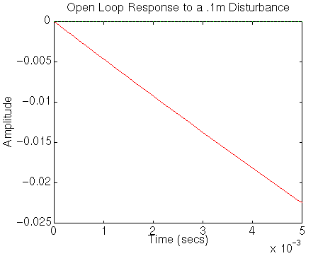
step(A,.1*B,C,D,2,0:0.0001:.005);

This plot shows that the spring, K1 compresses very quickly, and exceeds our requirement of 5mm in response to a .1m step after only a little more than 0.001s. Therefore, we will set T=.0005s in order to give the controller a chance to respond.

Continuous to Discrete Conversion

Now that we have selected a sampling time, we can convert the plant to discrete time. Matlab can be used to convert the above state space model, A,B,C, and D, to a discrete state space model, Ad,Bd,Cd, and Dd, by using c2dm command. The c2dm command can take six arguments: the four state matrices, the sampling time, T, and the type of hold circuit. In this example we will use zero-order hold ('zoh'). Refer to the Digital Control Tutorials page for more information.

Add the following code to your m-file:

T=.0005;
[Ad Bd Cd Dd]=c2dm(A,B,C,D,T,'zoh')

Matlab should return the following:


Ad =

    1.0000    0.0005    0.0000    0.0000
   -0.0035    1.0000   -0.0124   -0.0001
    0.0234    0.0000    0.9760    0.0005
    0.7705    0.0002   -0.9112    0.9998


Bd =

    0.0000    0.0000
    0.0000    0.0035
    0.0000   -0.0234
    0.0000   -0.7705


Cd =

     0     0     1     0


Dd =

     0     0

which represent the new discrete-time state space model.

Adding an Integrator

In this example, we will need to add an integrator to the system in order to drive the steady-state response to zero. We will add this integrator in series with the plant. This will have the effect of adding another state to the plant. We will add the integrator by representing it in state space and the using the series command. This command takes the A,B,C, and D matrices of the two systems to be connected in series as arguments and returns a new set of A,B,C, and D matrices. An integrator in discrete time state space can be represented as a trapezoidal approximation of integration over each sample period as follows:

To add this, add the following commands in your m-file:

Ai=1;
Bi=1;
Ci=T;
Di=T/2;

[Ada,Bda,Cda,Dda]=series(Ad,Bd,Cd,Dd,Ai,Bi,Ci,Di)

Matlab will return a new set of integrator-augmented state matrices, with dimension 5 rather than dimension 4. Unfortunately, the output of these equations is now the new integrated state. We must change the output Cda matrix to output the original output state. Add the following line:

Cda=[Cd 0]

Since the augmented state is the last state, this outputs the same state as the unaugmented equations.

Designing the Controller

The structure of the controller is similar to the structure of the continuous-time state space controller. We will now use the place command to compute the gain matrix, K, which will, in feedback, give us sny desired closed-loop poles.

We first need to decide where to place the closed-loop poles. Since we get to place all five of the closed-loop poles, we can be very selective about where to place them. In particular, we can place them to cancel all of the plant zeros, as well as give us the desired response. First, we will find the plant zeros by converting the plant's digital state equations to a transfer function, and then finding the roots of the numerator. We will use the ss2tf command which takes the state matrices and the selected input as arguments and outputs a transfer function numerator and denominator.

Add the following code to your m-file:

[num,den]=ss2tf(Ad,Bd,Cd,Dd,1);
zeros=roots(num)

Matlab will return the following:


zeros =

   0.9986 + 0.0065i
   0.9986 - 0.0065i
  -0.9929

We will select these three zeros as three of our desired closed-loop poles. One of the other two will be selected at .9992 since a pole there settles in approximately 10000 samples (or 5 seconds). The last pole will be selected at z=.2 since this is sufficiently fast to be insignificant. Add the following code to your m-file:

p1=.97+.13i;
p2=.97-.13i;
p3=-.87;
p1=zeros(1);
p2=zeros(2);
p3=zeros(3);
p4=.9992;
p5=.5;

K=place(Ada,Bda*[1;0],[p1 p2 p3 p4 p5])

Matlab will return the following:


place: ndigits= 19

K =

   1.0e+09 *

    0.0548    0.0000    1.0897    0.0011    0.0009

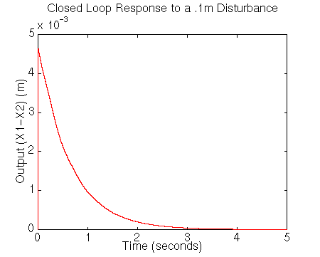
Simulating the Closed-Loop Response

We can use the dstep command to simulate the closed-loop response. Since multiplying the state vector by K in our controller only returns a single signal, u, we need to add a row of zeros to K by multiplying it by [1 0]^T. This is identical to what was done in the continuous design to compensate for the fact that there are two inputs to the plant, but only one is a control input. We will simulate with a negative .1m step disturbance in the road to give us a positive deflection of the bus for aesthetic reasons. Enter the following code into your m-file:

yout=dstep(Ada-Bda*[1 0]'*K,-.1*Bda,Cda,-.1*Dda,2,10001);
t=0:.0005:5;
stairs(t,yout);

You should see the following plot.

We can see in this plot, that the overshoot is less than 5mm, and the response settles well within 5 seconds.

User Feedback

8/24/97 JL
8/24/97 WM