

|
|
Plotting the frequency response using the bode
command
Adding a two-lead controller
Plotting the closed-loop response
From the main problem, the dynamic equations in transfer function form are the
following:


and the system schematic is:
For the original problem and the derivation of the above equations and schematic, please refer to the bus modeling page.
We want to design a feedback controller so that when the road disturbance (W) is simulated by a unit step input, the output (X1-X2) has a settling time less than 5 seconds and an overshoot less than 5%. For example, when the bus runs onto a 10 cm high step, the bus body will oscillate within a range of +/- 5 mm and will stop oscillating within 5 seconds.
The system model can be represented in Matlab by creating a new m-file and entering the following commands (refer to the main problem for the details of getting those commands).
m1=2500;
m2=320;
k1 = 80000;
k2 = 500000;
b1 = 350;
b2 = 15020;

nump=[(m1+m2) b2 k2]
denp=[(m1*m2) (m1*(b1+b2))+(m2*b1) (m1*(k1+k2))+(m2*k1)+(b1*b2) (b1*k2)+(b2*k1) k1*k2]

num1=[-(m1*b2) -(m1*k2) 0 0]
den1=[(m1*m2) (m1*(b1+b2))+(m2*b1) (m1*(k1+k2))+(m2*k1)+(b1*b2) (b1*k2)+(b2*k1) k1*k2]

numf=num1;
denf=nump;
The main idea of frequency-based design is to use the Bode plot of the open-loop transfer function to estimate the closed-loop response. Adding a controller to the system changes the open-loop Bode plot so that the closed-loop response will also change. Let's first draw the Bode plot for the original open-loop transfer function. Add the following line of code to your m-file and rerun:
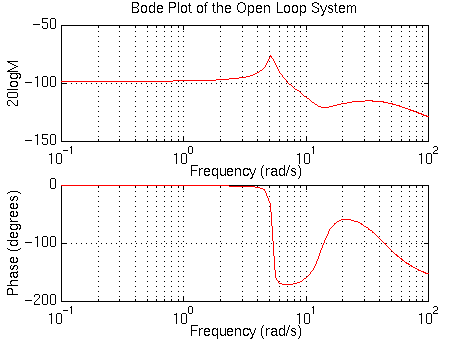
For convenience in representing systems with different natural frequencies of the system, we normalize and scale our finding before plotting the Bode plot, so that the low-frequency asymptote of each term is at 0 dB. This normalization by adjusting the gain, K, makes it easier to add the components of the Bode plot. The effect of K is move the magnitude curve up (increasing K) or down (decreasing K) by an amount 20*logK, but the gain, K, has no effect on the phase curve. Therefore from the previous plot, K must be equal to 100 dB or 100,000 to move the magnitude curve up to 0 dB at 0.1 rad/s. Go back to your m-file and add the following line of code to your m-file before the bode command and rerun:
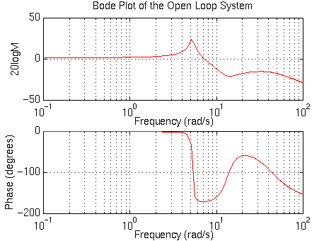
From the Bode plot above, we see that the phase curve is concave at about 5 rad/sec. First, we will try to add positive phase around this region, so that the phase will remain above the -180 degree line. Since a large phase margin leads to a small overshoot, we will want to add at least 140 degrees of positive phase at the area near 5 rad/sec. Since one lead controller can add no more than +90 degrees, we will use a two-lead controller:

To obtain T and a, the following steps can be used:
1: Determine the positive phase needed :

4: Determine T and aT from the following equations, these determine the corner frequencies so that the maximum phase will be added at the desired frequency.

Now let's put our 2-Lead controller into the system and see what the Bode plot looks like. Add the following code to your m-file, and add a % in front of the previous bode command (if there is one):
numc=conv([1.13426 1], [1.13426 1]);
denc=conv([0.035265 1], [0.035265 1]);
margin(conv(nump,numc),conv(denp,denc))
You should get the following Bode plot:
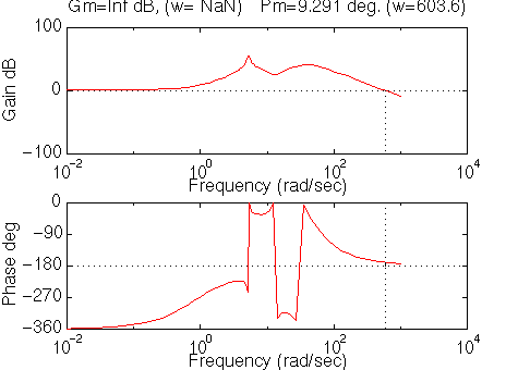
Since the Bode plot has a limited phase range (-360-0), the above plot is a little deceiving. The plot is equivalent to the following:
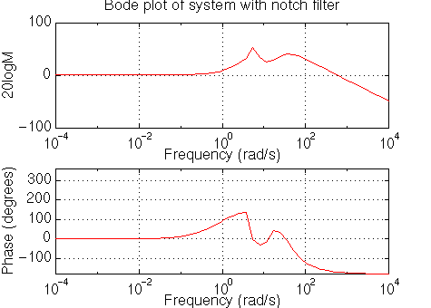
From this plot we see that the concave portion of the phase plot is above -180 degrees now, and the phase margin is large enough for the design criteria. Let's see how the output (the distance X1-X2) responds to a bump on the road (W). Recall that the schematic of the system is:
and the closed-loop transfer function can be derived as follows:
To obtain the closed-loop transfer function from W to X1-X2, the following commands can be added into the m-file:
numa=conv(conv(numf,nump),denc);
dena=conv(denf,polyadd(conv(denp,denc),conv(nump,numc)));
Note that the function "polyadd" is not a Matlab standard function. You will need to copy it to a new m-file to use it. Click here for more information.
Refer to the bus modeling page, nump = denf as we can see in the matlab command above. Thus we can simplified this transfer function to be the following:
numa=conv(numf,denc);
dena=polyadd(conv(denp,denc),conv(nump,numc));
Let's see what the step response looks like now. Keep in mind that we are using a 0.1 m high step as the disturbance. To simulate this, simply multiply numa by 0.1. Add the following code into the m-file and rerun it. Don't forget to put % mark in front of all bode and margin commands!
t=0:0.01:5;
step(0.1*numa,dena,t)
axis([0 5 -.01 .01])
and you should see the following plot:
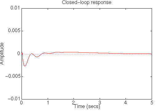
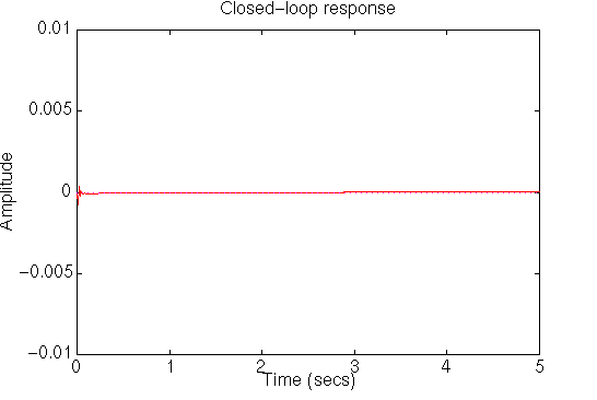
From this plot we can see that the percent overshoot is about 0.15 mm less than the previous plot's and the settling time also less than 5 seconds. This response is now satisfactory and no more design iteration is needed.
Tutorials